Introduction
Discovering 3D molecular structures for medicine or new materials has conventionally been done through human expertise. Modern Deep Learning techniques have proven to be a more efficient approach.
Generating 3D molecular structures that are both chemically valid and physically accurate is a critical challenge in computational chemistry and drug discovery. Traditional methods for molecular generation have relied on heuristic and rule-based approaches, which often lack the flexibility and generalizability required to handle the vast diversity of molecular structures. In the paper we based our project on, the use of a 3D Equivariant Diffusion Model (EDM) that has Graph Neural Networks, Diffusion Models and E(3) equivariant as key components, is introduced in order to leverage the symmetries to the Euclidean group in 3 dimensions that molecules have, outperforming previous 3D molecular generative models.
Motivation
The discovery of novel molecules is a crucial step in the development of new products that can be used for drug discovery for the treatment of complex diseases, developing material science and other molecular design related fields. But finding new chemical compounds with desired properties is a challenging task, as the space of synthesizable molecules is vast and sear in it proves to be very difficult, mostly owing to its discrete nature (Cao and Kipf, 2022). Although conventional molecular design involves the use of human expertise to propose, synthesize and test new molecules, this process can be cost and time intensive, limiting the number and diversity of molecules that can be reasonably explored (Bilodeau et al., 2022). Indeed, it has been estimated that the number of compounds that have ever been synthesized lies around while the total number of theoretically feasible compounds lies between and [(Polishchuk et al., 2013)].
In light of this situation, modern Deep Learning techniques provides an alternative and more efficient approach to achieve this through generative models. There are two characteristics of Deep Learning that makes it particularly promising when applied to molecules: First, they can cope with “unstructured” data representations such as text sequences, speech signals, images and graphs. Second, Deep Learning can perform feature extraction from the input data, that is, produce data-driven features from the input data without the need for manual intervention (Atz et al., 2021).
Background
Introduction to Graphs
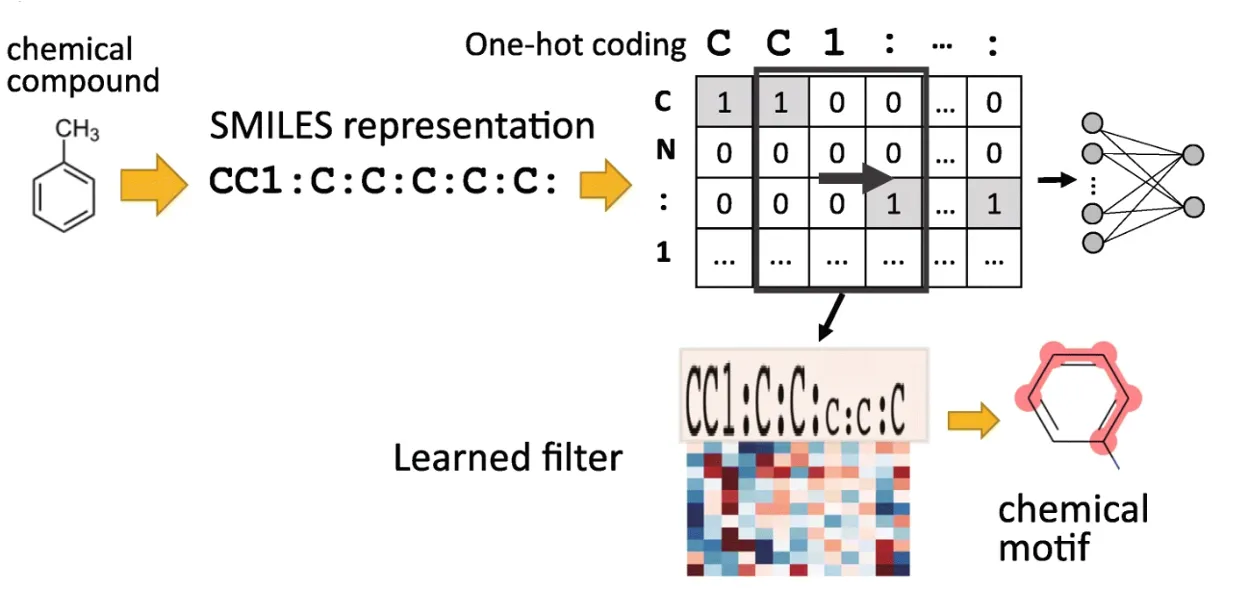
Concerning the use of Deep Learning techniques for molecules generation, according with (Maziarz et al., 2022), early approaches relied on the textual SMILES (Simplified molecular input line entry system) representation and on the reuse of architectures from Natural Language processing: treating molecules elements like atoms, bonds, etc. as the words of an NLP model.
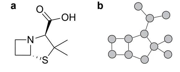
However, since 2018 we can observe the use of Graph Neural Networks (GNN) for this goal, as stated in (Cao and Kipf, 2022), due to the great improvements that were made on graphs in the area of deep learning during 2017 (Bronstein et al., 2017). Using graphs is convenient for this goal as this representation is able to encapsulate crucial structural information for molecules generation. Moreover, is has the benefit that all generated outputs are valid graphs (but not necessarily valid molecules).
Introduction to Diffusion Models
As we said, the paper we used as baseline, Hoogeboom et al. (2022), combines the use of GNN with Diffusion Models (DMs), standing as the first Diffusion Model that generates molecules in 3D space.
The use of Diffusion Models have gained more attention since the introduction of the Diffusion Probabilistic Models (DPMs) framework by Dhariwal and Nichol (2021) in 2020. They have shown remarkable success in generating high-quality data across various domains, including image synthesis and audio generation.
These models operate by iteratively denoising a sample starting from pure noise, guided by a learned probability distribution that captures the underlying structure of the target data.
In contrast to other generative models, in diffusion models the generative process is defined with respect to the true denoising process, which is known after modelling the reverse process of diffusion from a certain given data point .
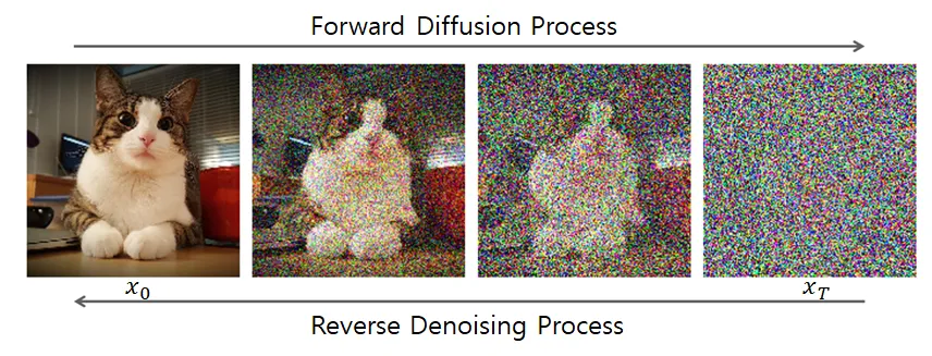
The diffusion process consists of progressively adding noise to for given a starting point by sampling from the multivariate normal distribution:
Where controls how much signal is retained and how much noise is added. As the diffusion process is Markov, the entire noising process can be written as:
Then, the posterior of the transitions conditioned on gives the true denoising process, which we can use to define our generative model:
and
with and , setting:
In fact, during the generative process, variable is unkown, so we replace it with an approximation given by a neural network .
Introduction to Equivariance transformations
The reason why using an equivariance approach for molecule generation is convenient lies on the inherent symmetries of molecular structures to those transformations. By leveraging symmetries, equivariant models can reduce redundant computations. For instance, once a particular arrangement is learned, its symmetric counterparts are automatically accounted for, which can lead to more efficient training and inference processes.
A function f is said to be equivariant to the action of a group G if:
Where are linear representations related to the group element (Serre (1977)). In this work, we only consider the Euclidean group E(3) generated by translations, rotations and reflections. We will have then that the function is equivariant to a translation and an orthogonal matrix that rotates or reflects coordinates if:
EDM: E(3) Equivariance Diffusion Model for molecules generation
The Equivariance Diffusion Model has the following four key points:
- It uses a generative diffusion process for molecules generation: models .
- The distribution from which noise, coordinates and features are sampled is E(n) invariant: use of center of gravity.
- The Neural Network that predicts coordinates and features for the distribution is E(n) equivariant: use of EGNN.
- It is easier to optimize the Neural Network if it predicts the Gaussian noise that is used for predicting and .
In this work interactions between all atoms are considered and model through a fully connected graph with nodes . Each node has associated a coordinate representation and an attribute vector .
In our case, we want the denoising distribution to be equivariant for the reasons discussed in the Introduction to Equivariance section, and thus, we want the denoising distribution from the introduction to diffusion section, to be equivariant. That distribution, applied to and will be:
Where we use a conventional normal distribution for the features because they are invariant to , and a normal distribution on the linear subspace where the center of gravity of is zero: , to lead with the non invariance of to such transformations.
Also, the neural network we use for approximiating and must be equivariant as well. For that, we use EGNN, a type of Graph Neural Network that satisfies the equivariance constraint.
The EGNN architecture is composed of L Equivariant Convolutional Layers EGCL layers wich applies non-linear transformation, that owe their equivariance to the fact that they use the coordinates difference among all nodes in the molecule.
According with Ho et al. (2020), it is actually easier to optimize the neural network when we predict the Gaussian noise of and instead, with such that:
Introduction to JAX
JAX is an open-source library for numerical computing that combines automatic differentiation with the capability to run code on GPUs and TPUs. Created by Google Research, JAX serves as a high-performance alternative to PyTorch and NumPy, enhanced by gradient-based optimization and just-in-time compilation.
JAX’s key features make it particularly effective for machine learning:
- NumPy Compatibility: JAX’s API is very similar to NumPy’s, making it easy for users to switch. Functions in JAX have the same names and signatures as those in NumPy.
- Automatic Differentiation: JAX includes powerful tools for automatic differentiation. The ‘grad’ function helps compute gradients of scalar-valued functions, and the ‘vjp’ and ‘jvp’ functions handle Jacobian-vector and vector-Jacobian products.
- Accelerator Support: JAX code can run on CPUs, GPUs, and TPUs with few changes, offering great versatility.
- Composable Function Transformations: JAX supports composable transformations like ‘grad’ for gradients, ‘jit’ for just-in-time compilation, ‘vmap’ for vectorization, and ‘pmap’ for parallelization across devices.
JIT paradigm
Just-In-Time (JIT) compilation is a standout feature in JAX. It optimizes code by converting Python functions into efficient machine code, which can be run on accelerators.
- JIT Usage: In JAX, the ‘@jit’ decorator marks functions for JIT compilation. When used, JAX employs the XLA compiler to turn the function into machine code. This involves tracing the function to create a computation graph, which XLA then compiles.
- Performance Impact: JIT compilation can greatly improve performance, especially for intensive tasks. By optimizing the computation graph and fusing operations, XLA cuts down on the overhead from Python’s dynamic nature and speeds up execution.
XLA
XLA (Accelerated Linear Algebra) is a specialized compiler that optimizes machine learning computations. It’s crucial to JAX’s performance and offers several benefits:
- Compilation Process: XLA processes the computation graph from JAX and optimizes it through operation fusion, constant folding, and kernel generation. These optimizations reduce memory use and speed up execution.
- Operation Fusion: XLA’s operation fusion combines multiple operations into a single kernel, reducing memory accesses and boosting computational efficiency.
Handling Graphs in JAX
JAX handles graphs efficiently despite their irregular data structures using several techniques:
- Padding Nodes and Edges: To batch process graphs, they are padded to a uniform size by adding dummy nodes and edges, ensuring all graphs in a batch have the same number of nodes and edges. This creates consistent tensor shapes for GPU processing.
- Masking: Masks, binary arrays indicating valid elements of padded tensors, ensure that padding doesn’t affect computation. Masks are applied to ignore padded elements during computation.
- Batch Processing: With padding and masking, graphs can be processed in batches for efficient GPU computation. JAX’s ‘vmap’ operations enhance this by automatically applying operations across batches.
Our contribution
Our contribution to this project had three goals:
- First, we reproduce the original E(3) Equivariance Diffusion Model (EDM).
- We rewrote the train and evaluation of the original paper using JAX. With this, we expect the model to be significantly faster than the original with similar results in terms of the metric: negative Log Likelihood.
- We experimented with our JAX version of the code by changing the number of diffusion steps that we jit together, comparing both run and compilation times.
Our primary contribution was meant to be re-implementing the original EDM from (Hogeboom (2022)) in the JAX/FLAX framework. JAX, with its ability to automatically differentiate through native Python and Numpy functions, and FLAX, which provides a high-level interface for neural network building, collectively offer significant advantages in terms of performance and flexibility.
By porting the model to JAX/FLAX, we aimed to:
- Improve Computational Efficiency: JAX’s just-in-time compilation and automatic vectorization capabilities can significantly speed up the training and inference processes.
- Enhance Scalability: The new implementation can leverage distributed computing resources more effectively, allowing for training on larger datasets and more complex models.
- Facilitate Research and Development: The modular and flexible nature of FLAX makes it easier for researchers to experiment with different model architectures and training regimes.
Besides rewriting the code in JAX, we also ran the original PyTorch code alongside the new JAX code to reproduce it and to compare results. Both code runs used the same hyperparameters, allowing for a direct comparison of performance and outcomes.
Finally, we wanted to test how do jitted functions affect the performance, and in order to evaluate it we measured the run and compilation time when we apply jit to a different number of timesteps during molecule generation.
Implementation
Our code is available in our repository and it is currently running.
To implement the model with JAX we made use of other libraries that are useful to build neural networks with JAX. Flax and Optax, that allow for an development process. Flax allows to create objects that mimic the pytorch nn.Module networks while not containing the parameters and other mutable variables as attributtes. Optax allows for ready to use optimizers.
Flax allows that the forward passes of the different modelues are similar to the pytorch version there is not much interest in the comparison of this part.
-
Generic Forward Pass:
-
JAX:
# Define Model Parameters def init_params(layer_sizes, key): keys = random.split(key, len(layer_sizes)) params = [(random.normal(k, (m, n)) * jnp.sqrt(2.0/m), jnp.zeros(n)) for m, n, k in zip(layer_sizes[:-1], layer_sizes[1:], keys)] return params # Define Model Functions def relu(x): return jnp.maximum(0, x) def forward(params, x): activations = x for W, b in params[:-1]: activations = relu(jnp.dot(activations, W) + b) final_W, final_b = params[-1] logits = jnp.dot(activations, final_W) + final_b return logits # Compute Forward Pass x = random.normal(key, (1, 784)) # Example input: batch size of 1 logits = forward(params, x) -
PyTorch:
# Define Model Class
class SimpleNN(nn.Module):
    def __init__(self, input_size, hidden_size, output_size):
        super(SimpleNN, self).__init__()
        self.fc1 = nn.Linear(input_size, hidden_size)
        self.fc2 = nn.Linear(hidden_size, output_size)

    def forward(self, x):
        x = F.relu(self.fc1(x))
        x = self.fc2(x)
        return x

# Initialize Model and compute Forward Pass
model = SimpleNN(input_size=784, hidden_size=128, output_size=10)

x = torch.randn(1, 784)  # Example input: batch size of 1
logits = model(x)
To see specific implementations of the EGNN and the difussion model see src/egnn/egnn.py, src/egnn/models.py and equivariant_diffusion/en_diffusion.py However, the backward pass is computed differently. In pytorch, after the forward pass and the computation of the loss, the gradient is calculated backtracking the operations and stored outputs of each calculation. In JAX, we define a loss function that depends on the parameters and then, the functional jax.grad is used to compute the gradient function of the loss with respect to the parameters. Then this gradient is evaluated on the parameters. This way, JAX generates the gradient function independently of the parameters so we can compile that gradient function straightforward to make it faster.
-
-
Backward pass:
-
JAX:
# Define Loss Function def loss(params, x, y): logits = forward(params, x) return jnp.mean(jnp.square(logits - y)) # Mean squared error loss # Compute Gradients x = random.normal(key, (1, 784)) # Example input y = random.normal(key, (1, 10)) # Example target output grad_loss = grad(loss) gradients = grad_loss(params, x, y) -
PyTorch:
# Defines Loss Function
criterion = nn.MSELoss()  # Mean squared error loss

# Compute Forward pass and Loss
x = torch.randn(1, 784)  # Example input
y = torch.randn(1, 10)   # Example target output

logits = model(x)
loss = criterion(logits, y)

# Compute Gradients
loss.backward()
Both approaches automatically handle differentiation. Again JAX uses a more functional approach, as opposed to the OOP style of PyTorch.
For more details on the backward pass and training step see src/train_test.py
-
—>
Results
1. Replication of the original E(3) Equivariant Diffusion Model
We compare results on the QM9 dataset with code from the original repository.
The replication yielded the following results:
| Metric | PyTorch (24-hour Run) |
|---|---|
| Training steps | 595641 |
| Validity | 89.4% |
| Atm stable | 97.73% |
| Mol stable | 74.1% |
| NLL | -97.29 |
While it was trained for a shorter time than reported in the paper, the results are agreeable, demonstrating a good reproducability.
Also, we were able to visualize the evolution of the molecules we generated through the generation process, as we can visualize in the following gif, which each frame represents the state of a certain molecule during each step of the denoising process:
2. Re-implementation of the code in JAX
In order to achieve this, we re-wrote most of the original repository in our own one, which can be found in this repository. Our implementation doesn’t contain all the files from the original repository, but the ones that are needed to run the training and validation steps.
Unfortunately, due to time constraints, we haven’t been able to run our implementation and get results. The code is able to train already, but there are still some unsolved bugs in the NLL calculation.
In order to verify the correctness of our implementation, we would run the original PyTorch code and our JAX implementation side by side, and compare the obtained models after 1000 epochs with the same hyperparameters as used in the original training procedure. While results are not identical due to differences between PyTorch and JAX, we expect them to be similar.
3. Experiments with the number of jit steps
The goal of this experiment was to find the best model speed by balancing run and compilation time, as the JIT paradigm gives us the possiblity of jit a certain number of training steps. However, the bigger the number of number of steps, the larger time compilation requires, for a potentially bigger speed boost. Therefore it is important to find the best balance between these two factors.
Unfortunately, the time constraints also affected this section and made us unable to run the experiments we wanted. Future work could investigate this further and provide a more detailed analysis of the impact of jit steps on model performance. Some interesting questions to answer would be:
- What is the trade-off between model speed and compilation time when using jit steps?
- Comparison of forward and backward pass times for different jit steps.
- How does the number of jit steps affect the model’s loss curve?
Conclusion
In conclusion, the E(3) Equivariant Diffusion Model represents a significant advancement in the field of molecular generation, providing a robust framework for generating 3D molecules with high fidelity.
Our re-implementation in JAX/Flax aims to further enhance the model’s efficiency and scalability, making it more accessible and practical for broader use in molecular sciences.
Contributions
- Harold: Reproduction of the original code. Debugging JAX code.
- Marina: Organisation and coordination of the project. Redaction of the blogpost’s introduction to theoretical approach, results and conclusion. Correction of the blogpost. README. Support with coding our JAX approach. Plot of results.
- Ricardo: JAX Code and JIT time steps experiment. Redaction of the blogpost’s Implementation to JAX.
- Robin: Blogspost setup. Redaction of the blogpost’s Introduction and Implementation to JAX. Blogspot review. README.